Synthesizing a population of binary stars

Dyad has a subpackage, dyad.stats, that contains probability distributions for the mass ratios and orbital elements of a population of binary stars. These probability distributions are implemented in the same way as Scipy’s continous random variables (see scipy.stats.rv_continuous and, for an example, scipy.stats.loguniform). As a result, they come equipped with a large number of useful methods, in particular pdf, which computes the probability density function (PDF), and rvs, which generates random variates (i.e. which generates a sample).

For example, consider the random variable for inclination, \(I\), which has PDF given by

\[\begin{split}f_{I}(i) = \begin{cases} \frac{1}{2}\sin(i) &\text{ if $i \in [0, \pi)$}\\ 0 &\text{ otherwise.} \end{cases}\end{split}\]

This random variable is implemented by Dyad using the class dyad.stats.inclination. Instantiate the class as follows.

>>> import dyad
>>> rv = dyad.stats.inclination

Now compute the PDF on the interval \([0, \pi)\).

>>> import numpy as np
>>> x = np.linspace(0., np.pi)
>>> pdf = rv.pdf(x)

And generate a sample of size \(10\,000\).

>>> sample = rv.rvs(size=10_000)

Now plot our results.

>>> import matplotlib.pyplot as plt
>>> fig, ax = plt.subplots()
>>> ax.hist(sample, bins="auto", density=True, histtype="stepfilled", alpha=0.2)
(array([0.04519806, 0.08320552, 0.12943081, 0.18798285, 0.24242597,
       0.22701754, 0.32768595, 0.36055726, 0.36774787, 0.39445581,
       0.42938159, 0.46430736, 0.43965387, 0.49615145, 0.49615145,
       0.53415891, 0.49306976, 0.49512422, 0.47868856, 0.43451773,
       0.44376279, 0.4406811 , 0.41089147, 0.34206715, 0.32357703,
       0.29995077, 0.27427006, 0.21160911, 0.18490116, 0.11607684,
       0.06882432, 0.0287624 ]), array([0.01702368, 0.11437298, 0.21172229, 0.3090716 , 0.40642091,
       0.50377021, 0.60111952, 0.69846883, 0.79581814, 0.89316744,
       0.99051675, 1.08786606, 1.18521536, 1.28256467, 1.37991398,
       1.47726329, 1.57461259, 1.6719619 , 1.76931121, 1.86666052,
       1.96400982, 2.06135913, 2.15870844, 2.25605775, 2.35340705,
       2.45075636, 2.54810567, 2.64545498, 2.74280428, 2.84015359,
       2.9375029 , 3.03485221, 3.13220151]), [<matplotlib.patches.Polygon object at 0x...>])
>>> ax.set_xticks([0., 0.5*np.pi, np.pi], [r"$0$", r"$\pi/2$", r"$\pi$"])
[<matplotlib.axis.XTick object at 0x...>, <matplotlib.axis.XTick object at 0x...>, <matplotlib.axis.XTick object at 0x...>]
>>> ax.set_xlabel(r"$i$")
Text(0.5, 0, '$i$')
>>> ax.set_ylabel(r"$f_{I}$")
Text(0, 0.5, '$f_{I}$')
>>> ax.plot(x, pdf)
[<matplotlib.lines.Line2D object at 0x...>]
>>> plt.show()

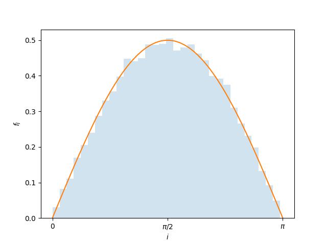
Fig. 5 The probability density function for inclination.

Some of Dyad’s random variables are dependent on other random variables. We must use their shape parameters to fully specify them. For example, the true anomaly of a body moving on an elliptical orbit in a gravitational central potential depends on that orbit’s eccentricity, so we are interested in the conditional distribution of \(\Theta\) given \(E\). Again, we can synthesize a sample and compute the PDF. Suppose that \(e = 0.5\).

>>> rv = dyad.stats.true_anomaly(e=0.5)
>>> x = np.linspace(0., 2.*np.pi)
>>> pdf = rv.pdf(x)
>>> sample = rv.rvs(size=10_000)

Then plot the results.

>>> fig, ax = plt.subplots()
>>> ax.hist(sample, bins="auto", density=True, histtype="stepfilled", alpha=0.2)
(array([0.04892705, 0.05045602, 0.04969153, 0.05580741, 0.06192329,
       0.06574572, 0.06192329, 0.07491954, 0.06956814, 0.07950645,
       0.08103542, 0.11620173, 0.11314379, 0.12690453, 0.13990077,
       0.17353812, 0.19953061, 0.21329134, 0.2614539 , 0.31879028,
       0.34478278, 0.36771733, 0.40441261, 0.39829673, 0.41358644,
       0.41587989, 0.33255102, 0.32949308, 0.29126882, 0.24463523,
       0.23163898, 0.19723715, 0.17277363, 0.13684283, 0.13760732,
       0.10626343, 0.10473446, 0.08944476, 0.08103542, 0.07950645,
       0.07033263, 0.04739808, 0.04434014, 0.04281117, 0.04816256,
       0.04892705, 0.0565719 , 0.04434014]), array([3.62268908e-03, 1.34429687e-01, 2.65236685e-01, 3.96043683e-01,
       5.26850681e-01, 6.57657679e-01, 7.88464677e-01, 9.19271675e-01,
       1.05007867e+00, 1.18088567e+00, 1.31169267e+00, 1.44249967e+00,
       1.57330666e+00, 1.70411366e+00, 1.83492066e+00, 1.96572766e+00,
       2.09653466e+00, 2.22734165e+00, 2.35814865e+00, 2.48895565e+00,
       2.61976265e+00, 2.75056965e+00, 2.88137664e+00, 3.01218364e+00,
       3.14299064e+00, 3.27379764e+00, 3.40460464e+00, 3.53541163e+00,
       3.66621863e+00, 3.79702563e+00, 3.92783263e+00, 4.05863963e+00,
       4.18944662e+00, 4.32025362e+00, 4.45106062e+00, 4.58186762e+00,
       4.71267462e+00, 4.84348161e+00, 4.97428861e+00, 5.10509561e+00,
       5.23590261e+00, 5.36670961e+00, 5.49751660e+00, 5.62832360e+00,
       5.75913060e+00, 5.88993760e+00, 6.02074460e+00, 6.15155159e+00,
       6.28235859e+00]), [<matplotlib.patches.Polygon object at 0x...>])
>>> ax.plot(x, pdf)
[<matplotlib.lines.Line2D object at 0x...>]
>>> ax.set_xticks([0., np.pi, 2.*np.pi], [r"$0$", r"$\pi$", r"$2\pi$"])
[<matplotlib.axis.XTick object at 0x...>, <matplotlib.axis.XTick object at 0x...>, <matplotlib.axis.XTick object at 0x...>]
>>> ax.set_xlabel(r"$\theta$")
Text(0.5, 0, '$\\theta$')
>>> ax.set_ylabel(r"$f_{\Theta}$")
Text(0, 0.5, '$f_{\\Theta}$')
>>> plt.show()

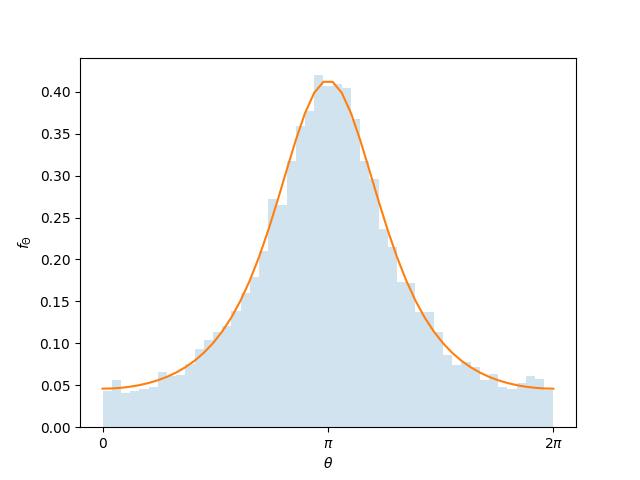
Fig. 6 The probability density function for true anomaly.

In some cases there is a choice of distribution. These are kept in the submodules dyad.stats.eccentricity, dyad.stats.log_period, dyad.stats.mass, dyad.stats.mass_ratio, dyad.stats.semimajor_axis. For example, when considering the eccentricity of an orbit we may wish to use a thermal distribution.

>>> rv = dyad.stats.eccentricity.thermal

Its methods are available in the same way as before.

>>> x = np.linspace(0., 1.)
>>> rv.pdf(x)
array([0.        , 0.04081633, 0.08163265, 0.12244898, 0.16326531,
       0.20408163, 0.24489796, 0.28571429, 0.32653061, 0.36734694,
       0.40816327, 0.44897959, 0.48979592, 0.53061224, 0.57142857,
       0.6122449 , 0.65306122, 0.69387755, 0.73469388, 0.7755102 ,
       0.81632653, 0.85714286, 0.89795918, 0.93877551, 0.97959184,
       1.02040816, 1.06122449, 1.10204082, 1.14285714, 1.18367347,
       1.2244898 , 1.26530612, 1.30612245, 1.34693878, 1.3877551 ,
       1.42857143, 1.46938776, 1.51020408, 1.55102041, 1.59183673,
       1.63265306, 1.67346939, 1.71428571, 1.75510204, 1.79591837,
       1.83673469, 1.87755102, 1.91836735, 1.95918367, 2.        ])

A complete population

Let us synthesize the complete orbital properties of a population of binary stars, namely the mass, mass ratio, and orbital elements. These have been determined for binary systems with sun-like primary stars in the solar neighbourhood by Duquennoy and Mayor [DM91]. According to Duquennoy and Mayor the mass ratio and period (which we can convert to semimajor axis) are independent of all other properties while the eccentricity is dependent on period. A system with period no longer than the circularization period of \(11.6~\text{d}\) has vanishing eccentricity (Sec. 7.2 Duquennoy and Mayor, 1991). Only a system with a period longer than this has an eccentricity that can be treated as a random variable. However, that random variable is itself dependent on period.

Dyad uses the distributions published by Duquennoy and Mayor to implement the random variables dyad.stats.mass_ratio.duquennoy1991, dyad.stats.log_period.duquennoy1991, and dyad.stats.eccentricity.duquennoy1991. Since eccentricity is dependent on period we must use its shape parameter, period, to fully specify it.

The primary stars in question have primary masses of \(M_{1}/\text{M}_{\odot} \in [0.9, 1.2]\) but the distributions of Duquennoy and Mayor are frequently assumed to hold for systems with red-giant primary stars, which have masses of \(0.8~\mathrm{M}_{\odot}\). Let us sample the mass ratio and the period for such a population.

>>> n = 10_000
>>> m_1 = np.full((n,), 0.8)
>>> q = dyad.stats.mass_ratio.duquennoy1991.rvs(size=n)
>>> p = 10.**dyad.stats.log_period.duquennoy1991.rvs(size=n)

Now sample the eccentricity, remembering that the circularization period is \(11.6~\mathrm{day}\).

>>> e = np.zeros(n)
>>> e[p > 11.6] = dyad.stats.eccentricity.duquennoy1991(p[p > 11.6]).rvs()

Using these eccentricities sample the true anomaly.

>>> theta = dyad.stats.true_anomaly(e).rvs()

Note that, since the eccentricities are all different, we do not pass a size argument to the method rvs. Now sample the orientation of the system.

>>> Omega = dyad.stats.longitude_of_ascending_node.rvs(size=n)
>>> i = dyad.stats.inclination.rvs(size=n)
>>> omega = dyad.stats.argument_of_pericentre().rvs(size=n)

The class dyad.TwoBody can serve as a container for these values. First convert the periods to their equivalent semimajor axes.

>>> a = dyad.semimajor_axis_from_period(p, m_1, m_1*q)

Then instantiate a dyad.TwoBody object.

>>> binary = dyad.TwoBody(m_1, m_1*q, a, e, Omega, i, omega)

We can now access the methods and attributes of binary.primary and binary.secondary. For example, their states.

>>> binary.primary.state(theta)
array([[ 9.80111287e+01,  9.32516010e+01,  3.07989658e+01,
         5.60306497e-05, -6.75192486e-05,  5.83210824e-05],
       [-4.22542976e-02,  5.26080375e-01,  1.14203942e+00,
         5.26000646e-05, -5.31249530e-05, -6.80699883e-06],
       [-6.81369019e-01, -2.01722338e-01,  1.34136797e-01,
        -2.89216118e-03, -1.49576197e-03, -6.95775004e-03],
       ...,
       [-2.54004074e+01,  1.95222411e+01,  2.83026032e+01,
         3.69555473e-04, -6.31504945e-04, -1.11761976e-04],
       [-4.90381509e+00,  1.69794112e+00,  1.85323362e+00,
        -1.21311936e-03, -1.18994396e-03, -1.14177399e-03],
       [-2.85454488e+02, -6.49690258e+02,  8.01143712e+02,
        -3.49444125e-05,  8.00978076e-05, -6.82733563e-05]])
>>> binary.secondary.state(theta)
array([[-3.22726839e+02, -3.07054870e+02, -1.01413513e+02,
        -1.84495319e-04,  2.22324485e-04, -1.92037158e-04],
       [ 1.21152600e+00, -1.50839108e+01, -3.27448458e+01,
        -1.50816247e-03,  1.52321221e-03,  1.95172007e-04],
       [ 7.53828180e-01,  2.23174195e-01, -1.48401372e-01,
         3.19972370e-03,  1.65482652e-03,  7.69766147e-03],
       ...,
       [ 3.34888768e+01, -2.57388756e+01, -3.73152437e+01,
        -4.87236190e-04,  8.32600476e-04,  1.47351299e-04],
       [ 8.15190285e+00, -2.82258829e+00, -3.08074023e+00,
         2.01664031e-03,  1.97811446e-03,  1.89803867e-03],
       [ 5.64217517e+02,  1.28415085e+03, -1.58350747e+03,
         6.90696782e-05, -1.58318009e-04,  1.34946288e-04]])

References

[DM91]

Duquennoy, A., and M. Mayor. 1991. 'Multiplicity among solar-type stars in the solar neighbourhood—II. Distribution of the orbital elements in an unbiased Sample'. Astronomy and Astrophysics 248 (August): 485.