Representing a Keplerian system

To a good approximation the Earth–Sun system is Keplerian. The Earth moves on an elliptical orbit with semimajor axis \(a = 1~\text{AU}\) and ellipticity \(e = 0.0167\) in the gravitational central potential generated by the Sun, which has mass \(m = 1~\text{M}_{\odot}\). We may represent this system in Dyad using the class dyad.Orbit.

>>> import dyad
>>> m, a, e = 1., 1., 0.0167
>>> orbit = dyad.Orbit(m, a, e)

The state (i.e. position and velocity) of the body is specified by its true anomaly, \(\theta\), which we can compute using the method dyad.Orbit.state. Suppose that \(\theta = 1\).

>>> theta = 1.
>>> orbit.state(theta)
array([ 0.53532139,  0.83371367,  0.        , -0.01447709,  0.00958295,
        0.        ])

This is given in the format \((x, y, z, v_{x}, v_{y}, v_{z})\) where \(x\), \(y\), and \(z\) are in units of \(\mathrm{AU}\) and \(v_{x}\), \(v_{y}\), and \(v_{z}\) are in units of \(\mathrm{AU}~\mathrm{d}^{-1}\). We can also compute the orbital radius and speed of the body, which are also in units of \(\mathrm{AU}\) and \(\mathrm{AU}~\mathrm{d}^{-1}\).

>>> orbit.radius(theta)
0.9907812427855317
>>> orbit.speed(theta)
0.017361418667972937

An instance of the class dyad.Orbit also has a number of attributes that represent constants of the orbit. These include the arguments with which dyad.Orbit was called.

>>> orbit.central_mass
1.0
>>> orbit.semimajor_axis
1.0
>>> orbit.eccentricity
0.0167

They also include more interesting constants, such as the period (in \(\mathrm{d}\)), periapsis (in \(\mathrm{AU}\)) and apoapsis (in \(\mathrm{AU}\)). A full list is available in the API documentation for dyad.Orbit.

>>> orbit.period
365.25689844815537
>>> orbit.periapsis
0.9833
>>> orbit.apoapsis
1.0167

If the perifocal frame differs from the observer’s frame we can specify its orientation using the Euler angles \(\Omega\), \(i\), and \(\omega\) (longitude of the ascending node, inclination, and argument of pericentre). Suppose that \(\Omega = 1\), \(i = 1\), and \(\omega = 1\).

>>> Omega, i, omega = 1., 1., 1.
>>> orbit = dyad.Orbit(m, a, e, Omega, i, omega)

All methods and attributes are available as before.

We may not always wish to work with true anomaly but instead prefer mean anomaly or eccentric anomaly. Dyad allows us to convert between these quantities.

>>> mu = dyad.mean_anomaly_from_true_anomaly(theta, e)
>>> dyad.true_anomaly_from_mean_anomaly(mu, e)
1.0
>>> eta = dyad.eccentric_anomaly_from_true_anomaly(theta, e)
>>> dyad.true_anomaly_from_eccentric_anomaly(eta, e)
1.0
>>> eta = dyad.eccentric_anomaly_from_mean_anomaly(mu, e)
>>> dyad.mean_anomaly_from_eccentric_anomaly(eta, e)
0.9720848452026836

To plot the evolution in time of any quantity first sample the mean anomaly uniformly on the interval \([0, 2\pi)\) and convert it to true anomaly. Consider, for example, the evolution of the orbital radius.

>>> import numpy as np
>>> mu = np.linspace(0., 2.*np.pi)
>>> theta = dyad.true_anomaly_from_mean_anomaly(mu, e)
>>> r = orbit.radius(theta)

Plot this.

>>> import matplotlib.pyplot as plt
>>> fig, ax = plt.subplots()
>>> ax.plot(mu/(2.*np.pi), r)
[<matplotlib.lines.Line2D object at 0x...>]
>>> ax.set_xlabel(r"$t/\mathrm{yr}$")
Text(0.5, 0, '$t/\\mathrm{yr}$')
>>> ax.set_ylabel(r"$r/\mathrm{au}$")
Text(0, 0.5, '$r/\\mathrm{au}$')
>>> plt.show()

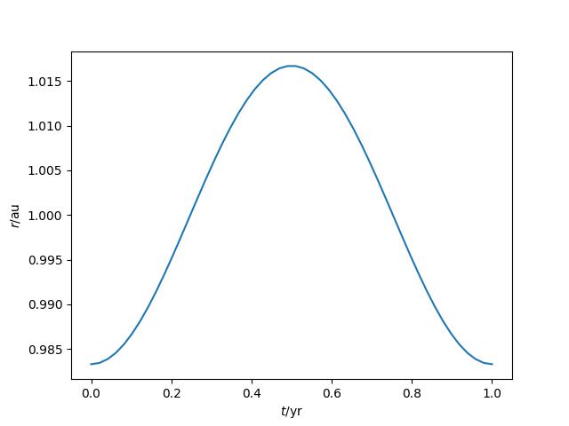
Fig. 4 The evolution of the Earth’s radius over the course of a year.

Delaunay elements

Given the central mass we may convert any set of orbital elements, \((a, e, \Omega, i, \omega, \theta)\) to the equivalent set of Delaunay elements, \((J_{1}, J_{2}, J_{3}, \Theta_{1}, \Theta_{2}, \Theta_{3})\) and vice versa. The functions are dyad.delaunay_elements_from_orbital_elements and dyad.orbital_elements_from_delaunay_elements. See the API documentation for the definitions used by Dyad.

Delaunay elements are not fully defined for \(e = 0\) or \(i = 0\) (as we have here) so we must instead use modified Delaunay elements, \((J_{\varpi}, J_{\Omega}, J_{\lambda}, \Theta_{\varpi}, \Theta_{\Omega}, \Theta_{\lambda})\). The functions are dyad.modified_delaunay_elements_from_orbital_elements and dyad.orbital_elements_from_modified_delaunay_elements. Again, see the API documentation for the definitions used by Dyad.

>>> m, a, e, Omega, i, omega, theta = 1., 1., 0.0167, 0., 0., 0., 1.
>>> dyad.modified_delaunay_elements_from_orbital_elements(a, e, Omega, i, omega, theta, m)
(2.398913957225284e-06, 0.0, 0.017202098944262438, -0.0, -0.0, 0.9720848452026836)
>>> dyad.orbital_elements_from_modified_delaunay_elements(*_, m)
(1.0, 0.01670000000000427, 0.0, 0.0, 0.0, 1.000000000000007)

In all threee cases (orbital elements, Delauany elements, and modified Delaunay elements) the first five elements define the orbit whilst the sixth defines the state. A list of the first five Delauanay elements is therefore available as a method of the dyad.Orbit class.

>>> orbit.modified_delaunay_elements()
array([ 2.39891396e-06,  7.90666244e-03,  1.72020989e-02, -2.00000000e+00,
       -1.00000000e+00])

We can use the keyword theta to specify the true anomaly. In this case the function then returns \(\Theta_{\lambda}\) also.

>>> orbit.modified_delaunay_elements(theta=1.)
array([ 2.39891396e-06,  7.90666244e-03,  1.72020989e-02, -2.00000000e+00,
       -1.00000000e+00,  2.97208485e+00])

Representing a binary system

To a good approximation the Alpha Centauri A–B system is an isolated binary. The two component stars have masses \(m_{A} = 1.0790~\text{M}_{\odot}\) and \(m_{B} = 0.9092~\text{M}_{\odot}\). The relative orbit has a semimajor axis \(a = 23.182~\text{AU}\) and an eccentricity \(e = 0.5195\). We may represent this system using the class dyad.TwoBody.

>>> import dyad
>>> m_A, m_B, a, e = 1.079, 0.9092, 23.182, 0.5195
>>> binary = dyad.TwoBody(m_A, m_B, a, e)

The properties of the relative orbit are available as an instance of the class dyad.Orbit with central mass \(m = m_{A} + m_{B}\). The class dyad.TwoBody has all the attributes of the class dyad.Orbit (see Representing a Keplerian system) plus three additional attributes: reduced_mass, primary, and secondary. The attribute reduced_mass holds the reduced mass of the secondary star, \(\mu = m_{1}m_{2}/(m_{1} + m_{2})\) while the attributes primary and secondary are themselves instances of the class Orbit and represent the properties of the primary and secondary stars’ orbits. The Orbit instance primary has the additional attribute mass, which holds the primary star mass. Similarly, the Orbit instance secondary has the additional attribute mass, which holds the secondary star mass.

>>> binary.reduced_mass
0.49342460517050596
>>> binary.primary
<dyad._core.Orbit object at 0x...>
>>> binary.secondary
<dyad._core.Orbit object at 0x...>

For example, we may find the state of the secondary star in coordinates relative to the primary as follows.

>>> binary.state(1.)
array([ 7.14066735e+00,  1.11209305e+01,  0.00000000e+00, -4.96110162e-03,
        6.24832826e-03,  0.00000000e+00])

The properties of the primary and secondary stars are represented in the in the observer’s frame, with the origin at the primary focus. They have masses as follows.

>>> binary.primary.mass
1.079
>>> binary.secondary.mass
0.9092

We may wish to know the orbital state of the two stars when \(\theta = 1\).

>>> binary.primary.state(1.)
array([ 3.26541331e+00,  5.08557992e+00,  0.00000000e+00, -2.26870214e-03,
        2.85734838e-03,  0.00000000e+00])
>>> binary.secondary.state(1.)
array([-3.87525403e+00, -6.03535056e+00, -0.00000000e+00,  2.69239948e-03,
       -3.39097988e-03, -0.00000000e+00])

We might also like to know the system’s other attributes. For example, the periods and periapses of the two stars.

>>> binary.primary.period
28913.10574161869
>>> binary.secondary.period
28913.105741618692
>>> binary.primary.periapsis
5.093820666532542
>>> binary.secondary.periapsis
6.045130333467458

Of course we might equivalently compute these last two values as follows.

>>> binary.primary.radius(0.)
5.093820666532543
>>> binary.secondary.radius(0.)
6.045130333467459

Note that all properties of the primary and secondary orbits are computed in the observer’s frame.