What is Dyad?

Dyad is a pure-Python two-body kinematics and binary-star statistics package for astrophysicists. It allows the user to compute the kinematic properties of a bound gravitational two-body system given that system’s physical properties (i.e. its component masses and orbital elements) and to synthesize a population of two-body systems with physical properties that follow a given distribution. Dyad allows the user to choose from a library of such distributions. This library includes (but is not limited to):

• the distributions of binary-star mass ratios and orbital elements published by Duquennoy and Mayor [DM91] and Moe and Stefano [MS17] and

• the distributions of initial stellar mass published by Kroupa [K02] and Salpeter [S55].

For a full list of available distributions see the API documentation for dyad.stats.

The basics

The geometry of an orbit is shown in Figures Fig. 1 and Fig. 2. That orbit is an ellipse with semimajor axis, \(a\) and eccentricity, \(e\). The body’s phase is described by its true anomaly, \(\theta\), which is the angle subtended by the body and the primary vertex (i.e. the point of perigee) at the primary focus, \(F_{1}\). The perifocal coordinate system has origin \(F_{1}\) and orthogonal basis \((\mathbf{e}_{p}, \mathbf{e}_{q}, \mathbf{e}_{w})\) such that \(\mathbf{e}_{p}\) is parallel with the latus rectum, \(\mathbf{e}_{q}\) is parallel with the major axis, and \(\mathbf{e}_{w}\) is parallel with the body’s angular momentum. If the observer’s frame is coordinatized by the orthogonal basis \((\mathbf{e}_{x}, \mathbf{e}_{y}, \mathbf{e}_{z})\) then the perifocal system is a rotation of the observer’s system defined by Euler angles \(\Omega\), \(i\), and \(\omega\) (being the longitude of the ascending node, the inclination, and the argument of pericentre).

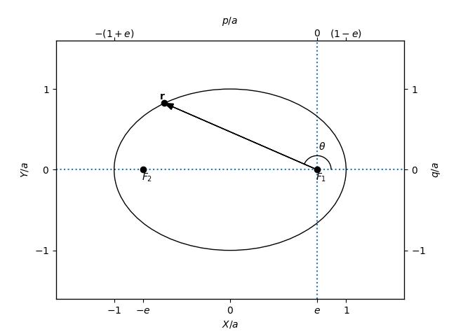
Fig. 1 The orbit of a bound body in a gravitational central potential. The pericentral frame has coordinates \(X\) and \(Y\) while the perifocal frame has coordinates \(p\) and \(q\).

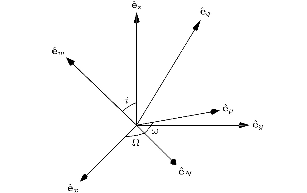
Fig. 2 The orientation of the perifocal coordinates system with respect to the coordinate system of the observer is described by the Euler angles \(\Omega\), \(i\), and \(\omega\). The unit vector \(\mathbf{e}_{N}\) is parallel with the line of nodes (i.e. the straight line passing through \(F_{1}\) and the ascending node, being the point at which the orbit and the observer’s plane of reference intersect).

The geometry of a binary system’s component orbits is shown in Figure Fig. 3. Both bodies move on elliptical orbits with primary foci coincident with the system’s centre of mass (COM) frame. The primary (resp. secondary) body moves as if in a central potential generated by a mass of \(m_{2}^{3}/(m_{1} + m_{2})^{2}\) (resp. \(m_{1}^{3}/(m_{1} + m_{2})^{2}\)). Its orbit is described by its semimajor axis, \(a_{1}\) (resp. \(a_{2}\)), and eccentricity, \(e_{1}\) (resp. \(e_{2}\)). Its orientation is defined by the longitude of its ascending node, \(\Omega_{1}\) (resp. \(\Omega_{2}\)), inclination, \(i_{1}\) (resp. \(i_{2}\)), and argument of pericentre, \(\omega_{1}\) (resp. \(\omega_{2}\)). The phase of the primary (resp. secondary) body is described by its true anomaly, \(\theta_{1}\) (resp. \(\theta_{2})\). It is the case that \(a_{2} = a_{1}/q\), \(e_{2} = e_{1}\). \(\Omega_{2} = \Omega_{1}\), \(i_{2} = i_{1}\), \(\omega_{2} = \omega_{1} + \pi\) and \(\theta_{1} = \theta_{2}\).

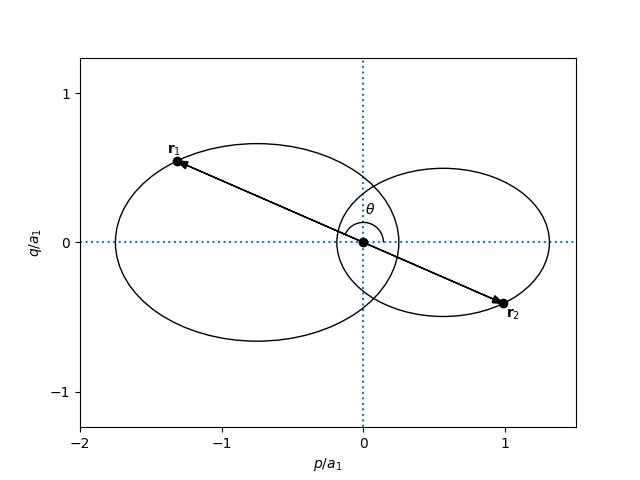
Fig. 3 The orbits of the components of a two-body system.

Units

Dyad uses the astronomical system of units: the unit of mass is solar mass, \(\mathrm{M}_{\odot}\), the unit of distance is the astronomical unit, \(\mathrm{AU}\), and the unit of time is the day, \(\mathrm{d}\). In this system the gravitational constant is \(\text{G} = 2.959122080881949 \times 10^{-4}~\text{M}_{\odot}~\text{d}^{2}~\text{AU}^{-3}\). Table 1 shows the units of several derived quantities and their equivalent SI values.

Table 1 The units of derived quantities in Dyad.

Quantity	Unit	Equivalent SI value
speed	\(\text{AU}~\text{d}^{-1}\)	\(1731456.8368055555~\text{m}~\text{s}^{-1}\)
action	\(\text{AU}^{2}~\text{d}^{-1}\)	\(2.590222559950685 \times 10^{17}~\text{m}^{2}~\text{s}^{-1}\)
potential	\(\text{AU}^{2}~\text{d}^{-2}\)	\(2997942777720.7007~\text{m}^{2}~\text{s}^{-2}\)
specific energy	\(\text{AU}^{2}~\text{d}^{-2}\)	\(2997942777720.7007~\text{m}^{2}~\text{s}^{-2}\)
specific angular momentum	\(\text{AU}^{2}~\text{d}^{-1}\)	\(2.590222559950685 \times 10^{17}~\text{m}^{2}~\text{s}^{-1}\)

References

[DM91]

Duquennoy, A., and M. Mayor. 1991. 'Multiplicity among solar-type stars in the solar neighbourhood—II. Distribution of the orbital elements in an unbiased Sample'. Astronomy and Astrophysics 248 (August): 485.

[MS17]

Moe, M., and R. Di Stefano. 2017. 'Mind your Ps and Qs: the interrelation between period (P) and mass-ratio (Q) distributions of binary stars.' The Astrophysical Journal Supplement Series 230 (2): 15.

[K02]

Kroupa, P. 2002. 'The initial mass function and its variation (review)'. ASP conference series 285 (January): 86.

[S55]

Salpeter, E. E. 1955. 'The luminosity function and stellar evolution.' The Astrophysical Journal 121 (January): 161.